The least squares method is one of the most common and most developed due to its simplicity and efficiency of methods for estimating the parameters of linear. At the same time, certain caution should be observed when using it, since the models built using it may not meet a number of requirements for the quality of their parameters and, as a result, not “well” reflect the patterns of process development.

Let us consider the procedure for estimating the parameters of a linear econometric model using the least squares method in more detail. Such a model in general form can be represented by equation (1.2):

y t = a 0 + a 1 x 1 t +...+ a n x nt + ε t .

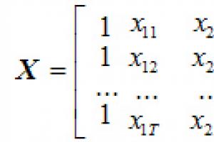
The initial data when estimating the parameters a 0 , a 1 ,..., a n is the vector of values ​​of the dependent variable y= (y 1 , y 2 , ... , y T)" and the matrix of values ​​of independent variables

in which the first column, consisting of ones, corresponds to the coefficient of the model .

The method of least squares got its name based on the basic principle that the parameter estimates obtained on its basis must satisfy: the sum of squares of the model error should be minimal.

Examples of solving problems by the least squares method

Example 2.1. The trading enterprise has a network consisting of 12 stores, information on the activities of which is presented in Table. 2.1.

The company's management would like to know how the size of the annual depends on the sales area of ​​the store.

Table 2.1

Shop number	Annual turnover, million rubles	Trade area, thousand m 2

Least squares solution. Let us designate - the annual turnover of the -th store, million rubles; - selling area of ​​the -th store, thousand m 2.

Fig.2.1. Scatterplot for Example 2.1

To determine the form of the functional relationship between the variables and construct a scatterplot (Fig. 2.1).

Based on the scatter diagram, we can conclude that the annual turnover is positively dependent on the selling area (i.e., y will increase with the growth of ). The most appropriate form of functional connection is − linear.

Information for further calculations is presented in Table. 2.2. Using the least squares method, we estimate the parameters of the linear one-factor econometric model

Table 2.2

Thus,

Therefore, with an increase in the trading area by 1 thousand m 2, other things being equal, the average annual turnover increases by 67.8871 million rubles.

Example 2.2. The management of the enterprise noticed that the annual turnover depends not only on the sales area of ​​the store (see example 2.1), but also on the average number of visitors. The relevant information is presented in table. 2.3.

Table 2.3

Solution. Denote - the average number of visitors to the th store per day, thousand people.

To determine the form of the functional relationship between the variables and construct a scatterplot (Fig. 2.2).

Based on the scatter diagram, we can conclude that the annual turnover is positively related to the average number of visitors per day (i.e., y will increase with the growth of ). The form of functional dependence is linear.

Rice. 2.2. Scatterplot for example 2.2

Table 2.4

In general, it is necessary to determine the parameters of the two-factor econometric model

y t \u003d a 0 + a 1 x 1 t + a 2 x 2 t + ε t

The information required for further calculations is presented in Table. 2.4.

Let us estimate the parameters of a linear two-factor econometric model using the least squares method.

Thus,

Evaluation of the coefficient = 61.6583 shows that, other things being equal, with an increase in the trading area by 1 thousand m 2, the annual turnover will increase by an average of 61.6583 million rubles.

Example.

Experimental data on the values ​​of variables X And at are given in the table.

As a result of their alignment, the function

Using least square method, approximate these data with a linear dependence y=ax+b(find options A And b). Find out which of the two lines is better (in the sense of the least squares method) aligns the experimental data. Make a drawing.

The essence of the method of least squares (LSM).

The problem is to find the linear dependence coefficients for which the function of two variables A And b takes the smallest value. That is, given the data A And b the sum of the squared deviations of the experimental data from the found straight line will be the smallest. This is the whole point of the least squares method.

Thus, the solution of the example is reduced to finding the extremum of a function of two variables.

Derivation of formulas for finding coefficients.

A system of two equations with two unknowns is compiled and solved. Finding partial derivatives of a function with respect to variables A And b, we equate these derivatives to zero.

We solve the resulting system of equations by any method (for example substitution method or ) and obtain formulas for finding the coefficients using the least squares method (LSM).

With data A And b function takes the smallest value. The proof of this fact is given.

That's the whole method of least squares. Formula for finding the parameter a contains the sums , , , and the parameter n- amount of experimental data. The values ​​of these sums are recommended to be calculated separately. Coefficient b found after calculation a.

It's time to remember the original example.

Solution.

In our example n=5. We fill in the table for the convenience of calculating the amounts that are included in the formulas of the required coefficients.

The values ​​in the fourth row of the table are obtained by multiplying the values ​​of the 2nd row by the values ​​of the 3rd row for each number i.

The values ​​in the fifth row of the table are obtained by squaring the values ​​of the 2nd row for each number i.

The values ​​of the last column of the table are the sums of the values ​​across the rows.

We use the formulas of the least squares method to find the coefficients A And b. We substitute in them the corresponding values ​​from the last column of the table:

Hence, y=0.165x+2.184 is the desired approximating straight line.

It remains to find out which of the lines y=0.165x+2.184 or better approximates the original data, i.e. to make an estimate using the least squares method.

Estimation of the error of the method of least squares.

To do this, you need to calculate the sums of squared deviations of the original data from these lines And , a smaller value corresponds to a line that better approximates the original data in terms of the least squares method.

Since , then the line y=0.165x+2.184 approximates the original data better.

Graphic illustration of the least squares method (LSM).

Everything looks great on the charts. The red line is the found line y=0.165x+2.184, the blue line is , the pink dots are the original data.

What is it for, what are all these approximations for?

I personally use to solve data smoothing problems, interpolation and extrapolation problems (in the original example, you could be asked to find the value of the observed value y at x=3 or when x=6 according to the MNC method). But we will talk more about this later in another section of the site.

Proof.

So that when found A And b function takes the smallest value, it is necessary that at this point the matrix of the quadratic form of the second-order differential for the function was positive definite. Let's show it.

Choosing the type of regression function, i.e. the type of the considered model of the dependence of Y on X (or X on Y), for example, a linear model y x = a + bx, it is necessary to determine the specific values ​​of the coefficients of the model.

For different values ​​of a and b, it is possible to construct an infinite number of dependencies of the form y x =a+bx, i.e., there are an infinite number of lines on the coordinate plane, but we need such a dependence that corresponds to the observed values ​​in the best way. Thus, the problem is reduced to the selection of the best coefficients.

We are looking for a linear function a + bx, based only on a certain number of available observations. To find the function with the best fit to the observed values, we use the least squares method.

Denote: Y i - the value calculated by the equation Y i =a+bx i . y i - measured value, ε i =y i -Y i - difference between the measured and calculated values, ε i =y i -a-bx i .

The method of least squares requires that ε i , the difference between the measured y i and the values ​​of Y i calculated from the equation, be minimal. Therefore, we find the coefficients a and b so that the sum of the squared deviations of the observed values ​​from the values ​​on the straight regression line is the smallest:

Investigating this function of arguments a and with the help of derivatives to an extremum, we can prove that the function takes on a minimum value if the coefficients a and b are solutions of the system:

(2)

If we divide both sides of the normal equations by n, we get:

Given that (3)

Get , from here, substituting the value of a in the first equation, we get:

In this case, b is called the regression coefficient; a is called the free member of the regression equation and is calculated by the formula:

The resulting straight line is an estimate for the theoretical regression line. We have:

So, is a linear regression equation.

Regression can be direct (b>0) and inverse (b Example 1. The results of measuring the X and Y values ​​are given in the table:

x i	-2	0	1	2	4
y i	0.5	1	1.5	2	3

Assuming that there is a linear relationship between X and Y y=a+bx, determine the coefficients a and b using the least squares method.

Solution. Here n=5
x i =-2+0+1+2+4=5;
x i 2 =4+0+1+4+16=25
x i y i =-2 0.5+0 1+1 1.5+2 2+4 3=16.5
y i =0.5+1+1.5+2+3=8

and normal system (2) has the form

Solving this system, we get: b=0.425, a=1.175. Therefore y=1.175+0.425x.

Example 2. There is a sample of 10 observations of economic indicators (X) and (Y).

x i	180	172	173	169	175	170	179	170	167	174
y i	186	180	176	171	182	166	182	172	169	177

It is required to find a sample regression equation Y on X. Construct a sample regression line Y on X.

Solution. 1. Let's sort the data by values ​​x i and y i . We get a new table:

x i	167	169	170	170	172	173	174	175	179	180
y i	169	171	166	172	180	176	177	182	182	186

To simplify the calculations, we will compile a calculation table in which we will enter the necessary numerical values.

x i	y i	x i 2	x i y i
167	169	27889	28223
169	171	28561	28899
170	166	28900	28220
170	172	28900	29240
172	180	29584	30960
173	176	29929	30448
174	177	30276	30798
175	182	30625	31850
179	182	32041	32578
180	186	32400	33480
∑x i =1729	∑y i =1761	∑x i 2 299105	∑x i y i =304696
x=172.9	y=176.1	x i 2 =29910.5	xy=30469.6

According to formula (4), we calculate the regression coefficient

and by formula (5)

Thus, the sample regression equation looks like y=-59.34+1.3804x.
Let's plot the points (x i ; y i) on the coordinate plane and mark the regression line.

Fig 4

Figure 4 shows how the observed values ​​are located relative to the regression line. To numerically estimate the deviations of y i from Y i , where y i are observed values, and Y i are values ​​determined by regression, we will make a table:

x i	y i	Y i	Y i -y i
167	169	168.055	-0.945
169	171	170.778	-0.222
170	166	172.140	6.140
170	172	172.140	0.140
172	180	174.863	-5.137
173	176	176.225	0.225
174	177	177.587	0.587
175	182	178.949	-3.051
179	182	184.395	2.395
180	186	185.757	-0.243

Y i values ​​are calculated according to the regression equation.

The noticeable deviation of some observed values ​​from the regression line is explained by the small number of observations. When studying the degree of linear dependence of Y on X, the number of observations is taken into account. The strength of the dependence is determined by the value of the correlation coefficient.

I am a computer programmer. I made the biggest leap in my career when I learned to say: "I do not understand anything!" Now I am not ashamed to tell the luminary of science that he is giving me a lecture, that I do not understand what it, the luminary, is talking to me about. And it's very difficult. Yes, it's hard and embarrassing to admit you don't know. Who likes to admit that he does not know the basics of something. By virtue of my profession, I have to attend a large number of presentations and lectures, where, I confess, in the vast majority of cases I feel sleepy, because I do not understand anything. And I don’t understand because the huge problem of the current situation in science lies in mathematics. It assumes that all students are familiar with absolutely all areas of mathematics (which is absurd). To admit that you do not know what a derivative is (that this is a little later) is a shame.

But I've learned to say that I don't know what multiplication is. Yes, I don't know what a subalgebra over a Lie algebra is. Yes, I do not know why quadratic equations are needed in life. By the way, if you are sure that you know, then we have something to talk about! Mathematics is a series of tricks. Mathematicians try to confuse and intimidate the public; where there is no confusion, no reputation, no authority. Yes, it is prestigious to speak in the most abstract language possible, which is complete nonsense in itself.

Do you know what a derivative is? Most likely you will tell me about the limit of the difference relation. In the first year of mathematics at St. Petersburg State University, Viktor Petrovich Khavin me defined derivative as the coefficient of the first term of the Taylor series of the function at the point (it was a separate gymnastics to determine the Taylor series without derivatives). I laughed at this definition for a long time, until I finally understood what it was about. The derivative is nothing more than just a measure of how much the function we are differentiating is similar to the function y=x, y=x^2, y=x^3.

I now have the honor of lecturing students who afraid mathematics. If you are afraid of mathematics - we are on the way. As soon as you try to read some text and it seems to you that it is overly complicated, then know that it is badly written. I argue that there is not a single area of ​​mathematics that cannot be spoken about "on fingers" without losing accuracy.

The challenge for the near future: I instructed my students to understand what a linear-quadratic controller is. Don't be shy, waste three minutes of your life, follow the link. If you do not understand anything, then we are on the way. I (a professional mathematician-programmer) also did not understand anything. And I assure you, this can be sorted out "on the fingers." At the moment I do not know what it is, but I assure you that we will be able to figure it out.

So, the first lecture that I am going to give to my students after they come running to me in horror with the words that the linear-quadratic controller is a terrible bug that you will never master in your life is least squares methods. Can you solve linear equations? If you are reading this text, then most likely not.

So, given two points (x0, y0), (x1, y1), for example, (1,1) and (3,2), the task is to find the equation of a straight line passing through these two points:

illustration

This straight line should have an equation like the following:

Here alpha and beta are unknown to us, but two points of this line are known:

You can write this equation in matrix form:

Here we should make a lyrical digression: what is a matrix? A matrix is ​​nothing but a two-dimensional array. This is a way of storing data, no more values ​​​​should be given to it. It is up to us how exactly to interpret a certain matrix. Periodically, I will interpret it as a linear mapping, periodically as a quadratic form, and sometimes simply as a set of vectors. This will all be clarified in context.

Let's replace specific matrices with their symbolic representation:

Then (alpha, beta) can be easily found:

More specifically for our previous data:

Which leads to the following equation of a straight line passing through the points (1,1) and (3,2):

Okay, everything is clear here. And let's find the equation of a straight line passing through three points: (x0,y0), (x1,y1) and (x2,y2):

Oh-oh-oh, but we have three equations for two unknowns! The standard mathematician will say that there is no solution. What will the programmer say? And he will first rewrite the previous system of equations in the following form:

In our case, the vectors i, j, b are three-dimensional, therefore, (in the general case) there is no solution to this system. Any vector (alpha\*i + beta\*j) lies in the plane spanned by the vectors (i, j). If b does not belong to this plane, then there is no solution (equality in the equation cannot be achieved). What to do? Let's look for a compromise. Let's denote by e(alpha, beta) how exactly we did not achieve equality:

And we will try to minimize this error:

Why a square?

We are looking not just for the minimum of the norm, but for the minimum of the square of the norm. Why? The minimum point itself coincides, and the square gives a smooth function (a quadratic function of the arguments (alpha,beta)), while just the length gives a function in the form of a cone, non-differentiable at the minimum point. Brr. Square is more convenient.

Obviously, the error is minimized when the vector e orthogonal to the plane spanned by the vectors i And j.

Illustration

In other words: we are looking for a line such that the sum of the squared lengths of the distances from all points to this line is minimal:

UPDATE: here I have a jamb, the distance to the line should be measured vertically, not orthographic projection. the commenter is right.

Illustration

In completely different words (carefully, poorly formalized, but it should be clear on the fingers): we take all possible lines between all pairs of points and look for the average line between all:

Illustration

Another explanation on the fingers: we attach a spring between all data points (here we have three) and the line that we are looking for, and the line of the equilibrium state is exactly what we are looking for.

Quadratic form minimum

So, given the vector b and the plane spanned by the columns-vectors of the matrix A(in this case (x0,x1,x2) and (1,1,1)), we are looking for a vector e with a minimum square of length. Obviously, the minimum is achievable only for the vector e, orthogonal to the plane spanned by the columns-vectors of the matrix A:

In other words, we are looking for a vector x=(alpha, beta) such that:

I remind you that this vector x=(alpha, beta) is the minimum of the quadratic function ||e(alpha, beta)||^2:

Here it is useful to remember that the matrix can be interpreted as well as the quadratic form, for example, the identity matrix ((1,0),(0,1)) can be interpreted as a function of x^2 + y^2:

quadratic form

All this gymnastics is known as linear regression.

Laplace equation with Dirichlet boundary condition

Now the simplest real problem: there is a certain triangulated surface, it is necessary to smooth it. For example, let's load my face model:

The original commit is available. To minimize external dependencies, I took the code of my software renderer, already on Habré. To solve the linear system, I use OpenNL , it's a great solver, but it's very difficult to install: you need to copy two files (.h + .c) to your project folder. All smoothing is done by the following code:

For (int d=0; d<3; d++) { nlNewContext(); nlSolverParameteri(NL_NB_VARIABLES, verts.size()); nlSolverParameteri(NL_LEAST_SQUARES, NL_TRUE); nlBegin(NL_SYSTEM); nlBegin(NL_MATRIX); for (int i=0; i<(int)verts.size(); i++) { nlBegin(NL_ROW); nlCoefficient(i, 1); nlRightHandSide(verts[i][d]); nlEnd(NL_ROW); } for (unsigned int i=0; i&face = faces[i]; for (int j=0; j<3; j++) { nlBegin(NL_ROW); nlCoefficient(face[ j ], 1); nlCoefficient(face[(j+1)%3], -1); nlEnd(NL_ROW); } } nlEnd(NL_MATRIX); nlEnd(NL_SYSTEM); nlSolve(); for (int i=0; i<(int)verts.size(); i++) { verts[i][d] = nlGetVariable(i); } }

X, Y and Z coordinates are separable, I smooth them separately. That is, I solve three systems of linear equations, each with the same number of variables as the number of vertices in my model. The first n rows of matrix A have only one 1 per row, and the first n rows of vector b have original model coordinates. That is, I spring-tie between the new vertex position and the old vertex position - the new ones shouldn't be too far away from the old ones.

All subsequent rows of matrix A (faces.size()*3 = the number of edges of all triangles in the grid) have one occurrence of 1 and one occurrence of -1, while the vector b has zero components opposite. This means I put a spring on each edge of our triangular mesh: all edges try to get the same vertex as their starting and ending points.

Once again: all vertices are variables, and they cannot deviate far from their original position, but at the same time they try to become similar to each other.

Here is the result:

Everything would be fine, the model is really smoothed, but it moved away from its original edge. Let's change the code a little:

For (int i=0; i<(int)verts.size(); i++) { float scale = border[i] ? 1000: 1; nlBegin(NL_ROW); nlCoefficient(i, scale); nlRightHandSide(scale*verts[i][d]); nlEnd(NL_ROW); }

In our matrix A, for the vertices that are on the edge, I add not a row from the category v_i = verts[i][d], but 1000*v_i = 1000*verts[i][d]. What does it change? And this changes our quadratic form of the error. Now a single deviation from the top at the edge will cost not one unit, as before, but 1000 * 1000 units. That is, we hung a stronger spring on the extreme vertices, the solution prefers to stretch others more strongly. Here is the result:

Let's double the strength of the springs between the vertices:
nlCoefficient(face[ j ], 2); nlCoefficient(face[(j+1)%3], -2);

It is logical that the surface has become smoother:

And now even a hundred times stronger:

What is this? Imagine that we have dipped a wire ring in soapy water. As a result, the resulting soap film will try to have the smallest curvature as possible, touching the same border - our wire ring. This is exactly what we got by fixing the border and asking for a smooth surface inside. Congratulations, we have just solved the Laplace equation with Dirichlet boundary conditions. Sounds cool? But in fact, just one system of linear equations to solve.

Poisson equation

Let's have another cool name.

Let's say I have an image like this:

Everyone is good, but I don't like the chair.

I'll cut the picture in half:

And I will select a chair with my hands:

Then I will drag everything that is white in the mask to the left side of the picture, and at the same time I will say throughout the whole picture that the difference between two neighboring pixels should be equal to the difference between two neighboring pixels of the right image:

For (int i=0; i

Here is the result:

Real life example

I deliberately did not do licked results, because. I just wanted to show exactly how you can apply the least squares methods, this is a training code. Let me now give a real life example:

I have a number of photographs of fabric samples like this one:

My task is to make seamless textures from photos of this quality. First, I (automatically) look for a repeating pattern:

If I cut out this quadrangle right here, then because of the distortions, the edges will not converge, here is an example of a pattern repeated four times:

Hidden text

Here is a fragment where the seam is clearly visible:

Therefore, I will not cut along a straight line, here is the cut line:

Hidden text

And here is the pattern repeated four times:

Hidden text

And its fragment to make it clearer:

Already better, the cut did not go in a straight line, bypassing all sorts of curls, but still the seam is visible due to uneven lighting in the original photo. This is where the least squares method for the Poisson equation comes to the rescue. Here's the final result after lighting alignment:

The texture turned out perfectly seamless, and all this automatically from a photo of a very mediocre quality. Do not be afraid of mathematics, look for simple explanations, and you will be lucky in engineering.

The problem is to find the linear dependence coefficients for which the function of two variables A And b takes the smallest value. That is, given the data A And b the sum of the squared deviations of the experimental data from the found straight line will be the smallest. This is the whole point of the least squares method.

Thus, the solution of the example is reduced to finding the extremum of a function of two variables.

Derivation of formulas for finding coefficients. A system of two equations with two unknowns is compiled and solved. Finding partial derivatives of functions by variables A And b, we equate these derivatives to zero.

We solve the resulting system of equations by any method (for example, the substitution method or the Cramer method) and obtain formulas for finding the coefficients using the least squares method (LSM).

With data A And b function takes the smallest value.

That's the whole method of least squares. Formula for finding the parameter a contains the sums , , , and the parameter n- amount of experimental data. The values ​​of these sums are recommended to be calculated separately. Coefficient b found after calculation a.

The main area of ​​application of such polynomials is the processing of experimental data (the construction of empirical formulas). The fact is that the interpolation polynomial constructed from the values ​​of the function obtained with the help of the experiment will be strongly influenced by "experimental noise", moreover, during interpolation, the interpolation nodes cannot be repeated, i.e. you can not use the results of repeated experiments under the same conditions. The root-mean-square polynomial smoothes the noise and makes it possible to use the results of multiple experiments.

Numerical integration and differentiation. Example.

Numerical Integration- calculation of the value of a definite integral (as a rule, approximate). Numerical integration is understood as a set of numerical methods for finding the value of a certain integral.

Numerical differentiation– a set of methods for calculating the value of the derivative of a discretely given function.

Integration

Formulation of the problem. Mathematical statement of the problem: it is necessary to find the value of a certain integral

where a, b are finite, f(x) is continuous on [а, b].

When solving practical problems, it often happens that the integral is inconvenient or impossible to take analytically: it may not be expressed in elementary functions, the integrand can be given in the form of a table, etc. In such cases, numerical integration methods are used. Numerical integration methods use the replacement of the area of ​​a curvilinear trapezoid by a finite sum of areas of simpler geometric shapes that can be calculated exactly. In this sense one speaks of the use of quadrature formulas.

Most methods use the representation of the integral as a finite sum (quadrature formula):

The quadrature formulas are based on the idea of ​​replacing the graph of the integrand on the integration interval with functions of a simpler form, which can be easily integrated analytically and, thus, easily calculated. The simplest task of constructing quadrature formulas is realized for polynomial mathematical models.

Three groups of methods can be distinguished:

1. Method with division of the segment of integration into equal intervals. The division into intervals is done in advance, usually the intervals are chosen equal (to make it easier to calculate the function at the ends of the intervals). Calculate areas and sum them up (methods of rectangles, trapezoid, Simpson).

2. Methods with partitioning of the segment of integration using special points (Gauss method).

3. Calculation of integrals using random numbers (Monte Carlo method).

Rectangle method. Let the function (drawing) be integrated numerically on the segment . We divide the segment into N equal intervals. The area of ​​each of the N curvilinear trapezoids can be replaced by the area of ​​a rectangle.

The width of all rectangles is the same and equal to:

As a choice of the height of the rectangles, you can choose the value of the function on the left border. In this case, the height of the first rectangle will be f(a), the second one will be f(x 1),…, N-f(N-1).

If we take the value of the function on the right border as the choice of the height of the rectangle, then in this case the height of the first rectangle will be f (x 1), the second - f (x 2), ..., N - f (x N).

As can be seen, in this case one of the formulas gives an approximation to the integral with an excess, and the second with a deficiency. There is another way - to use the value of the function in the middle of the integration segment for approximation:

Estimation of the absolute error of the method of rectangles (middle)

Estimation of the absolute error of the methods of left and right rectangles.

Example. Calculate for the entire interval and dividing the interval into four sections

Solution. Analytical calculation of this integral gives I=arctg(1)–arctg(0)=0.7853981634. In our case:

1) h = 1; xo = 0; x1 = 1;

2) h = 0.25 (1/4); x0 = 0; x1 = 0.25; x2 = 0.5; x3 = 0.75; x4 = 1;

We calculate by the method of left rectangles:

We calculate by the method of right rectangles:

Calculate by the method of average rectangles:

Trapezoidal method. Using a polynomial of the first degree for interpolation (a straight line drawn through two points) leads to the trapezoid formula. The ends of the integration segment are taken as interpolation nodes. Thus, the curvilinear trapezoid is replaced by an ordinary trapezoid, the area of ​​\u200b\u200bwhich can be found as the product of half the sum of the bases and the height

In the case of N segments of integration for all nodes, except for the extreme points of the segment, the value of the function will be included in the total sum twice (since neighboring trapezoids have one common side)

The trapezoid formula can be obtained by taking half the sum of the rectangle formulas along the right and left edges of the segment:

Checking the stability of the solution. As a rule, the shorter the length of each interval, i.e. the greater the number of these intervals, the less the difference between the approximate and exact values ​​of the integral. This is true for most functions. In the trapezoid method, the error in calculating the integral ϭ is approximately proportional to the square of the integration step (ϭ ~ h 2). Thus, to calculate the integral of a certain function in the limits a, b, it is necessary to divide the segment into N 0 intervals and find the sum of the areas of the trapezoid. Then you need to increase the number of intervals N 1, again calculate the sum of the trapezoid and compare the resulting value with the previous result. This should be repeated until (N i) until the specified accuracy of the result (convergence criterion) is reached.

For the rectangle and trapezoid methods, usually at each iteration step, the number of intervals increases by a factor of 2 (N i +1 =2N i).

Convergence criterion:

The main advantage of the trapezoid rule is its simplicity. However, if the integration requires high precision, this method may require too many iterations.

Absolute error of the trapezoidal method rated as
.

Example. Calculate an approximately definite integral using the trapezoid formula.

a) Dividing the integration segment into 3 parts.
b) Dividing the segment of integration into 5 parts.

Solution:
a) By condition, the integration segment must be divided into 3 parts, that is.
Calculate the length of each segment of the partition: .

Thus, the general formula of trapezoids is reduced to a pleasant size:

Finally:

I remind you that the resulting value is an approximate value of the area.

b) We divide the integration segment into 5 equal parts, that is, . by increasing the number of segments, we increase the accuracy of calculations.

If , then the trapezoid formula takes the following form:

Let's find the partitioning step:
, that is, the length of each intermediate segment is 0.6.

When finishing the task, it is convenient to draw up all calculations with a calculation table:

In the first line we write "counter"

As a result:

Well, there really is a clarification, and a serious one!
If for 3 segments of the partition , then for 5 segments . If you take even more segment => will be even more accurate.

Simpson formula. The trapezoid formula gives a result that strongly depends on the step size h, which affects the accuracy of calculating a definite integral, especially in cases where the function is nonmonotonic. One can assume an increase in the accuracy of calculations if, instead of segments of straight lines replacing the curvilinear fragments of the graph of the function f(x), we use, for example, fragments of parabolas given through three neighboring points of the graph. A similar geometric interpretation underlies Simpson's method for calculating the definite integral. The entire integration interval a,b is divided into N segments, the length of the segment will also be equal to h=(b-a)/N.

Simpson's formula is:

remainder term

With an increase in the length of the segments, the accuracy of the formula decreases, therefore, to increase the accuracy, the composite Simpson formula is used. The entire integration interval is divided into an even number of identical segments N, the length of the segment will also be equal to h=(b-a)/N. The composite Simpson formula is:

In the formula, the expressions in brackets are the sums of the values ​​of the integrand, respectively, at the ends of the odd and even internal segments.

The remainder term of Simpson's formula is already proportional to the fourth power of the step:

Example: Calculate the integral using Simpson's rule. (Exact solution - 0.2)

Gauss method

Quadrature formula of Gauss. The basic principle of quadrature formulas of the second variety is visible from Figure 1.12: it is necessary to place the points in such a way X 0 and X 1 inside the segment [ a;b] so that the areas of the "triangles" in total are equal to the areas of the "segment". When using the Gauss formula, the initial segment [ a;b] is reduced to the interval [-1;1] by changing the variable X on

0.5∙(b– a)∙t+ 0.5∙(b + a).

Then , Where .

This substitution is possible if a And b are finite, and the function f(x) is continuous on [ a;b]. Gauss formula for n points x i, i=0,1,..,n-1 inside the segment [ a;b]:

, (1.27)

Where t i And Ai for various n are given in reference books. For example, when n=2 A 0 =A 1=1; at n=3: t 0 =t 2" 0.775, t 1 =0, A 0 =A 2" 0.555, A 1" 0.889.

Quadrature formula of Gauss

obtained with a weight function equal to one p(x)= 1 and nodes x i, which are the roots of the Legendre polynomials

Odds Ai easily calculated by formulas

i=0,1,2,...n.

The values ​​of nodes and coefficients for n=2,3,4,5 are given in the table

Order	Knots	Odds
n=2	x 1=0 x 0 =-x2=0.7745966692	A 1=8/9 A 0 = A 2=5/9
n=3	x 2 =-x 1=0.3399810436 x 3 =-x0=0.8611363116	A 1 =A 2=0.6521451549 A 0 = A 3=0.6521451549
n=4	x 2 = 0 x 3 = -x 1 = 0.5384693101 x 4 =-x 0 =0.9061798459	A 0 =0.568888899 A 3 =A 1 =0.4786286705 A 0 =A 4 =0.2869268851
n=5	x 5 = -x 0 =0.9324695142 x 4 = -x 1 =0.6612093865 x 3 = -x 2 =0.2386191861	A 5 =A 0 =0.1713244924 A 4 =A 1 =0.3607615730 A 3 =A 2 =0.4679139346

Example. Calculate the value using the Gauss formula for n=2:

Exact value: .

The algorithm for calculating the integral according to the Gauss formula provides not for doubling the number of microsegments, but for increasing the number of ordinates by 1 and comparing the obtained values ​​of the integral. The advantage of the Gauss formula is high accuracy with a relatively small number of ordinates. Disadvantages: inconvenient for manual calculations; must be stored in computer memory t i, Ai for various n.

The error of the Gauss quadrature formula on the segment will be at the same time For the formula of the remainder term will be where the coefficient α N decreases rapidly with growth N. Here

Gauss formulas provide high accuracy already with a small number of nodes (from 4 to 10). In this case, in practical calculations, the number of nodes ranges from several hundred to several thousand. We also note that the weights of Gaussian quadratures are always positive, which ensures the stability of the algorithm for calculating the sums